Hyperspectral Vision Basics
Deep dive into the backgrounds of Hyperspectral Vision
- Introduction
- Sensors and spectral ranges
- Spatial resolution and working distance
- Excitation and sample motion
- Data acquisition and preprocessing
- Machine learning methods and data evaluation
- Soft modeling vs. hard modeling
Introduction
Modern industrial processes require ever-improving optical inspection for the in-process evaluation and assessment of products. Over the past two decades, optical non-contact technologies have been developed which, under the collective term 'machine vision', have made a significant contribution to product or process evaluation. Nevertheless, many tasks remain unsolved, either because they could not be captured by grayscale or color cameras and are still assessed by trained employees using their eyes, or because only spectral single-channel sensors are used, for example, which cannot capture data from a larger area. Due to the increasing complexity in development and production, some requirements can no longer be solved satisfactorily with the existing methods of optical inspection and new approaches are required. One of these is (multi- or hyper-)spectral imaging. Integrated system solutions refer further to the industrial usage and are known commonly as Hyperspectral Vision.
Spectral imaging options
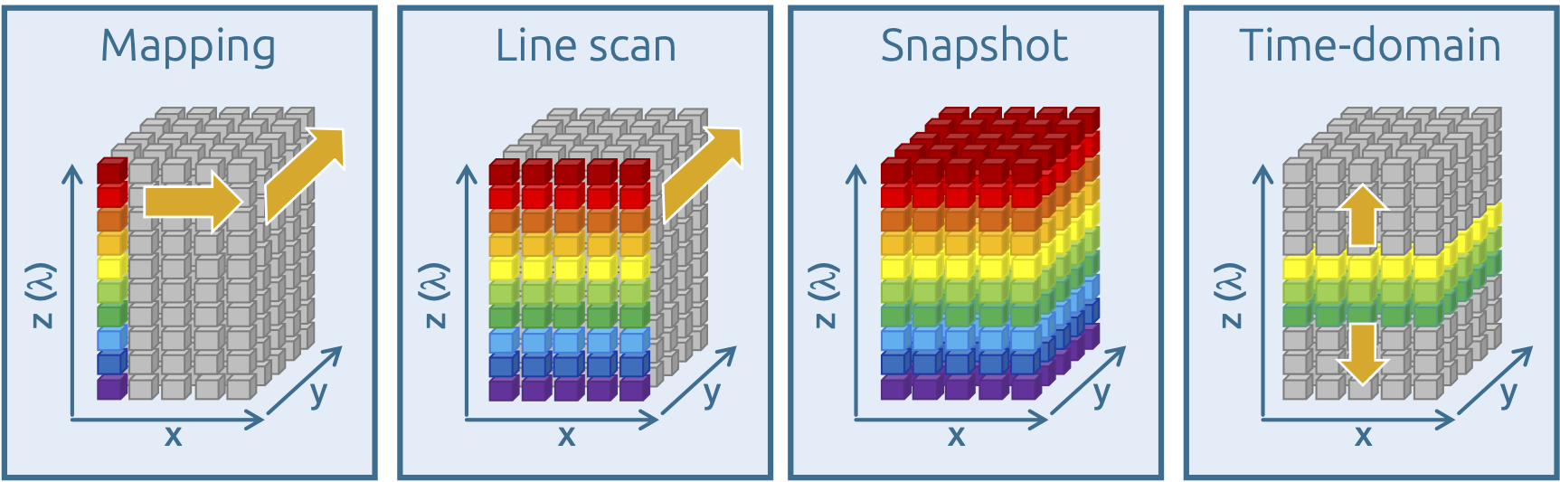
Spectral imaging has been established since the late 1960s, initially in satellite and aircraft-based remote sensing (including LANDSAT missions, Sojus missions/MKF6). Whereas a few spectral channels were initially recorded through optical filters, over 1000 spectral channels can now be recorded simultaneously. With laboratory spectrometers, on the other hand, spectral images were assembled point-by-point by mapping when computer-aided analysis began in the 1980s. Today's systems work either by sequentially recording spectrally resolved lines (pushbroom imager) or by recording the complete, spectrally resolved image (snapshot imager).
In most cases, line scan systems can offer the higher spectral resolution (hyperspectral), while real imaging tends to work with a few spectral bands (multispectral). An exception is so-called 'time-domain imaging' or 'spectral scanning', in which the spectral image is recorded along the wavelength axis.
In German-speaking countries, a distinction is made between multispectral and hyperspectral imaging (multispectral imaging/MSI; hyperspectral imaging/HSI):
- multispectral ≤ 100 spectral channels
- hyperspectral > 100 spectral channels
A multi- or hyperspectral system consists of: Illumination, optics/input slit, spectrometer, detector, data processing. The resulting data matrix of spectrally resolved images is the so-called 'hypercube'. In this setup, either the sample or the HSI system must be moved to record the hypercube. Depending on the inspection task, however, one of these two options is often available per se.
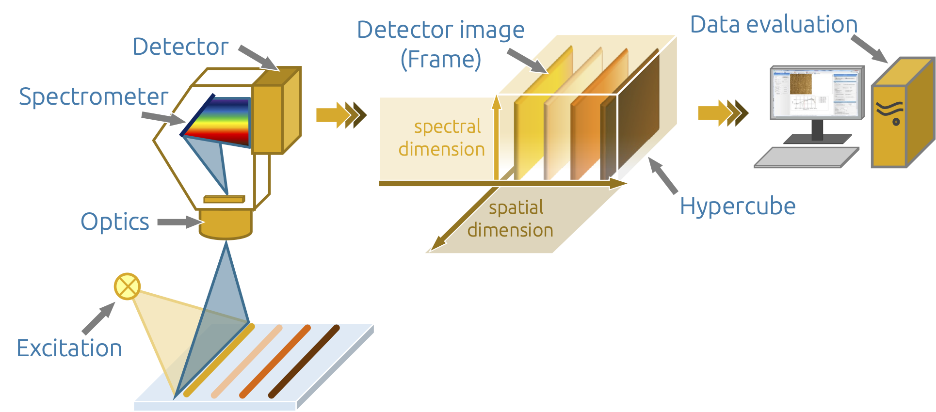
Scheme of a hyperspectral line scan imaging - 'pushbroom imaging'
Sensors and spectral ranges
In order to obtain a spectral dispersion, different spectrometer concepts are used for spectral imaging.
- Multispectral imaging:
- Multi-sensor: beam splitter and use of filters for several sensors; usually <10 spectral channels
- Multi-channel: spectral dispersion using special prisms with a spectral gradient filter; approx. 10-20 spectral channels
- Filter-on-chip: Fabry-Perot filters imprinted directly on the sensor chip; often 16 or 25 spectral channels (4x4 or 5x5 arrangement of channels)
- Hyperspectral imaging:
- Filter-on-chip: linear, spectral gradient filters applied directly to the sensor chip; often 100-200 spectral channels
- Holographic gratings in transmission or reflection (e.g. Offner setup); over 1000 spectral channels
The spectrometers used to date for hyperspectral imaging are all dispersive. They are less sensitive than conventional laboratory spectrometers, especially those based on the Fourier transform (FT) technique. However, the advantage of the systems lies in the use of spectral information in the area. Deviations in the area can be detected even with a poorer signal-to-noise ratio.
Just like the spectrometers of the HSI systems, the detectors are also tuned to a defined spectral range. Conventional silicon detectors (Si) are used for the spectral range from approx. 250 nm to approx. 1000 nm, while special semiconductor materials such as indium gallium arsenide (InGaAs) or mercury cadmium telluride (MCT) are used for the near infrared range above 1000 nm. Frequently used and commercially available spectral ranges for hyperspectral imaging are listed below.
- approx. 250 nm - 500 nm ultraviolet/visible (UV/VIS) with UV-enhanced silicon detector
- approx. 400 nm - 1000 nm visible/near-infrared (VIS/NIR; also known as VNIR) with silicon detector
- approx. 700 nm - 1600 nm near-infrared (NIR or SWIR for 'short wave infrared) with InGaAs detector
- approx. 1000 nm - 2500 nm near-infrared (NIR or SWIR for 'short wave infrared') with MCT detector
Depending on the detector, HSI systems now achieve up to 400 Hz at full resolution and >1000 Hz with binning or by selecting individual spectral channels (region of interest, ROI).
Spatial resolution and working distance
The optics/lenses of most HSI systems are variable, e.g. via the industry standard C-mount. This results in a wide range of configuration options, as illustrated in Fig. 3. The minimum working width of the HSI system is determined by the focal plane of the lens; in addition, the working distance (WD) can usually be freely selected. The resulting field of view (FOV) can therefore be set from a few millimetres (microscope) to several meters or kilometers.
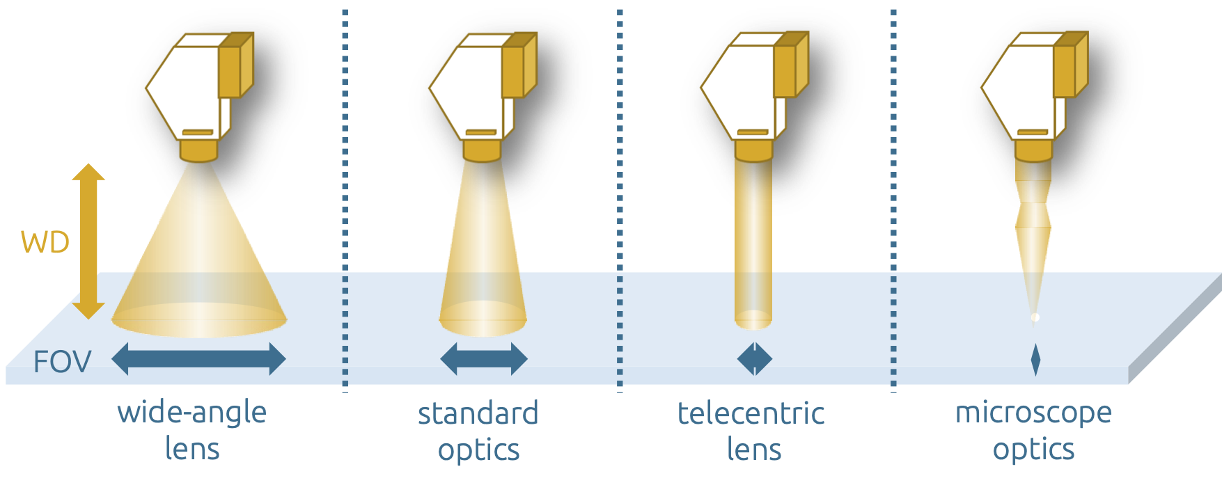
Hyperspectral imaging: field of view in different optics configurations
The theoretical spatial resolution of the scan line (x-coordinate) can be determined directly from the field of view and the available number of pixels of the detector; in reality, the resolution is also significantly influenced by the quality of the holographic grid. The spatial resolution of the y-coordinate, on the other hand, depends on the measurement parameters selected later, such as the measurement frequency of the detector and the speed of the samples. Therefore, hyperspectral data can have square pixels, but depending on the recording mode, the pixels can also be compressed or stretched. The spectral resolution (z-coordinate) depends on the combination of holographic grating, detector and input slit and is documented on the manufacturer's data sheets or calibration. When planning inspection tasks using HSI, it should also be taken into account that not all wavelengths can be imaged sharply at the same time due to the optics. The focal plane is not only shifted along the z-axis, but also by the wavelengths.
Excitation and sample motion
As with other spectral methods, hyperspectral imaging involves an interaction (absorption, reflection) of the light with the sample. For this reason, broadband sources are preferred for illumination. For the spectral ranges mentioned, these are, for example, halogen sources (VIS, NIR, SWIR) or deuterium lamps (UV). Depending on the sample morphology and structure, spot, line or diffuse illumination is selected. Special cases are transmission measurements and/or the recording of directional reflection, which are often found in microscope adaptations. The choice of the correct illumination is a decisive factor for successful hyperspectral measurements; in any case, the image line should be illuminated homogeneously. This is the only way to record reliable data and reduce the time and effort required for data evaluation or to enable meaningful data evaluation in the first place.
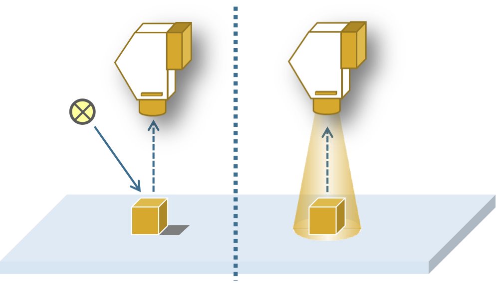
Schematic illustration of excitation with a spot source vs. diffuse excitation
While spot illumination tends to be influenced by the substrate (e.g. rolling direction of the stainless steel) and varying degrees of reflection of the primary beam, diffuse-homogeneous illumination enables observation of the aluminum oxide thin film applied to the stainless steel substrate. This is made possible by transferring the principle of the integrating sphere, which is well known in spectroscopy, to the illumination of the line. The Fraunhofer IWS has developed corresponding integration spheres for this purpose, which offer a corresponding diffuse-homogeneous light field through the use of optical PTFE (the sintered material creates many scattering centers). The working distances that can be realized with this are limiting, as the light is also scattered in all spatial directions at the exit slit.
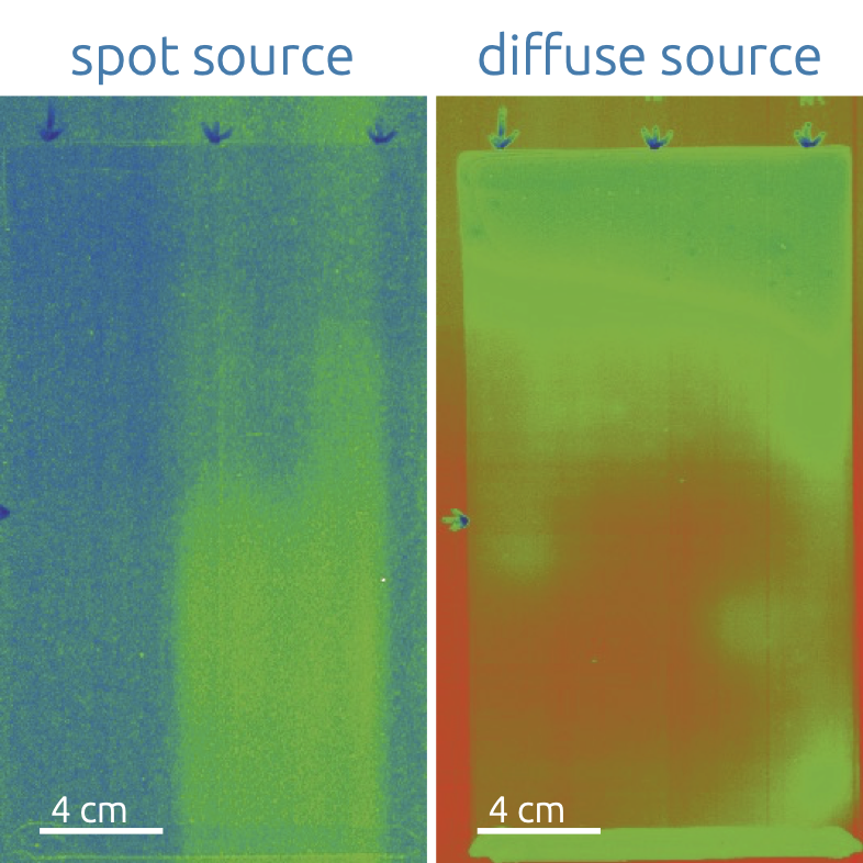
Example of differences caused by different excitation sources
For spherically larger samples (e.g. inspection of apples), 360° arrangements of individual spots are suitable as illumination in order to keep the intensity homogeneous at every point and every height of the sample. Fiber-coupled line or ring lights can also be used for samples that are less demanding in terms of their surface properties or size. However, the fibers used are often limited to the VIS range.
A motion system is also required to complete a measuring system. There are practically no limits to the possibilities from the laboratory and industrial environment, but the software for data acquisition should be synchronized with the respective motion system and the accuracy of the motion systems should meet the requirements of the sample or data acquisition. Options for motion systems include Linear, cross and rotary tables, conveyor belts, multi-axis gantries, robots.
Data acquisition and preprocessing
One of the most important tasks in preparation for data acquisition is to focus the object under investigation. The wavelength at which the detector has the highest sensitivity or quantum efficiency should initially be selected as the focal point. With known samples, it is of course also possible to focus on a defined wavelength (which is of particular interest for the evaluation). Particularly in the VNIR range, the possibility of binning (spectral and/or spatial summation of pixels on the detector) to increase intensity or minimize noise should also be examined. With higher intensities, in turn, the exposure time can be reduced and the recording frequency increased. In order to achieve a reliable evaluation of the hypercubes, necessary corrections such as bright and dark reference correction should already be carried out during data acquisition.

Typical spectroscopic corrections to avoid detector and system influences in measurements
Bright field correction (or white reference or background correction) is carried out, for example, on optical PTFE, silicon wafers or similar spectrally inert materials. Dark field correction removes the detector offset from the data. Missing pixel detection is also important for MCT detectors. This is used to spectrally interpolate defective pixels (light and dark pixels, indicators) on the detector.
Depending on the spectral resolution and spatial resolution, the resulting hypercubes can quickly reach sizes of several gigabytes. The way in which the hypercubes are viewed can vary: on the one hand, n images (with n = number of spectral bands/wavelengths) are available for data evaluation while on the other hand x*y spectra are available.
Since information acquisition in the area is desired and an unbeatable advantage of HSI technology, the reduction of the data volume in the spectral direction is initially favorable. The actual information of the spectra, which is necessary for further evaluation, is advantageously separated from the noise by mathematical transformations, thus reducing the amount of data.
The data pre-processing of the spectra therefore also works with the classic methods of spectroscopy, i.e:
- Baseline correction (e.g. linear, polynomial)
- Normalization (e.g. vector normalization, min/max normalization)
- Smoothing (e.g. Savitzky-Golay)
- Centering (e.g. mean value centering)
- Derivation(s)
For simpler questions, the user can get a first impression of which sample areas carry relevant information at which wavelengths by looking at individual wavelength images.
Machine learning methods and data evaluation
If a contextualization into a larger sample (or spectra) population is required or if correlations are to be examined that are not visible at first glance in individual samples, a machine learning approach respectively a mathematical-statistical evaluation of the data is therefore required, also known as a 'soft modeling' approach. After reducing the number of wavelengths or the description using feature images, methods of image evaluation and graphical pattern recognition, such as wavelet analysis, can describe structures in the surface using just a few parameters. In a final step, a regression model, for example, is used to classify the sample as a whole. In this way, extensive, complex raw data can be analyzed for a target value.
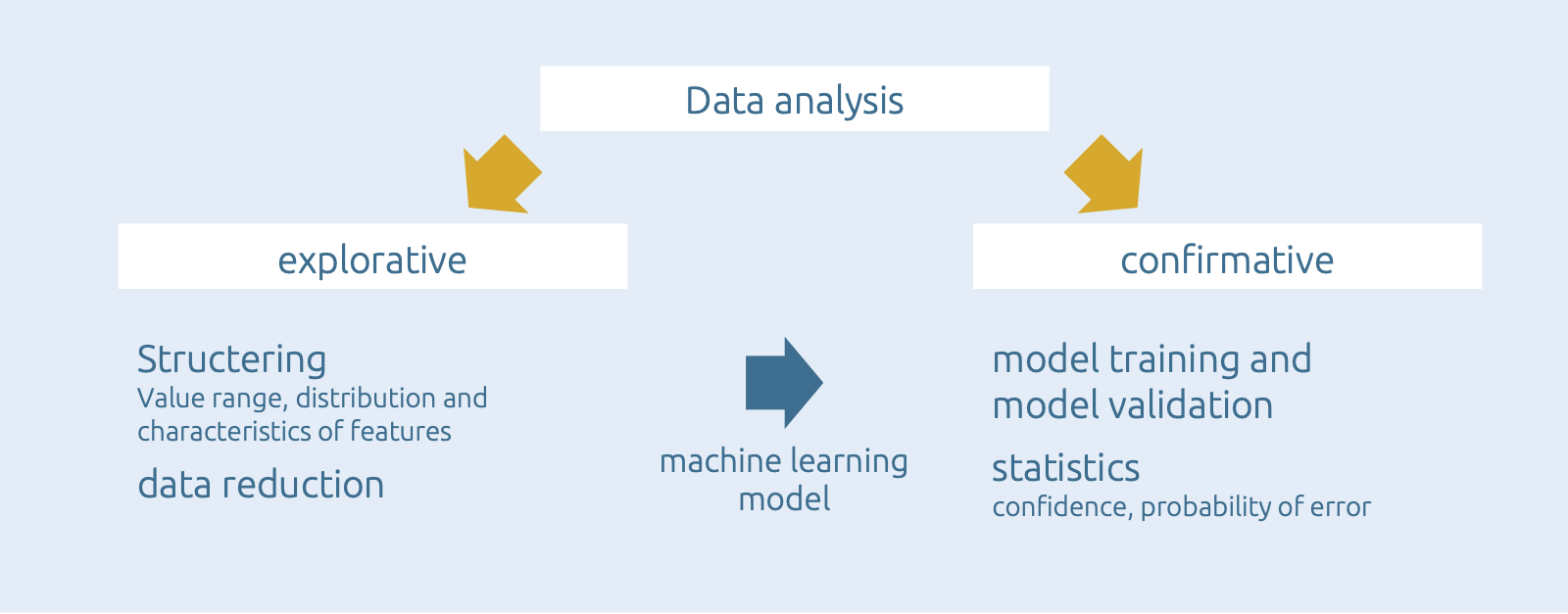
Schematically procedure for data analysis
The prerequisite for this procedure, however, is that a machine learning model is trained using reference samples with a known target value, which can be used for the subsequent prediction of the target value from unknown spectra or new samples. A distinction is made between continuous regression models and classification models with discrete assignment of the target value. This prediction can be automated in the process and can be carried out very quickly, optical inspection using Hyperspectral Vision technology is therefore also inline-capable.
If only the spectra totality is of interest and not their spatial distribution or the derivation of a target value, an evaluation and/or classification of the spectra or samples can also be carried out directly using methods of descriptive statistics or quantitative and qualitative multivariate data analysis (MVDA). Qualitative methods of MVDA are also suitable if the target value of a sample population is unknown or no reference exists. Frequently used methods are principle component analysis (PCA) and cluster analysis (CA).
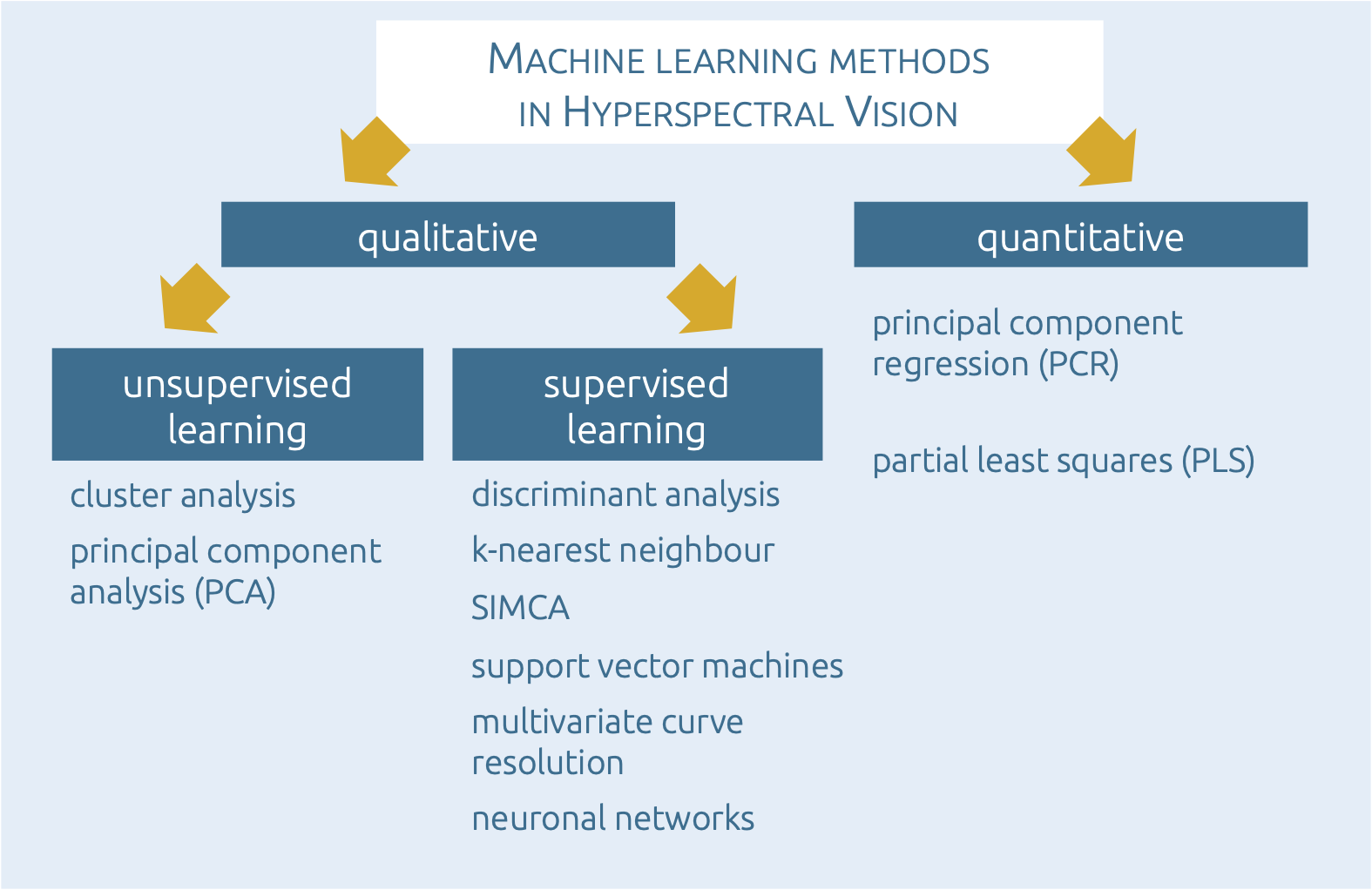
Common machine learning and AI methods for hyperspectral data analysis (non-exhaustive)
Soft modeling vs. hard modeling
In contrast to the machine learning methods of the 'soft modeling' approach, there is also the 'hard modeling' approach for evaluating the spectra. This refers to the physically exact description of the data. The simplest case is Lambert-Beer's law for describing the extinction. Other examples are the determination of optical properties (refractive index, absorption coefficient) and the sample structure (layer thicknesses) based on the description of the spectra using the laws of thin-film optics. The computing times required for hard modeling are significantly longer compared to the prediction in the soft modeling approach, but the results can also be used as a reference for classification or regression models.
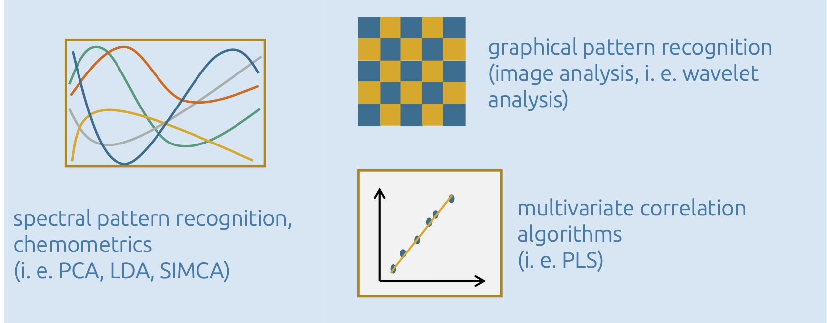
Examples for soft modeling algorithms
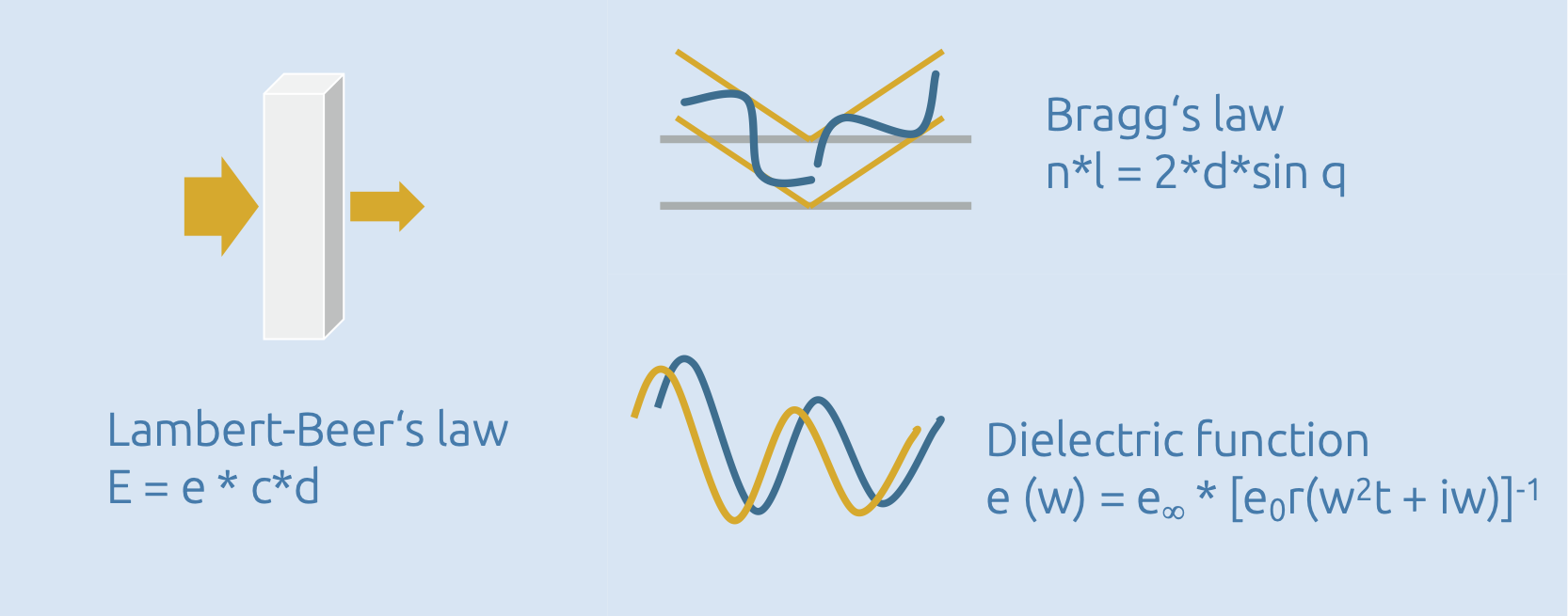
Examples for hard modeling algorithms